
An innovative simulation tool based on boundary integral equations (BIE) has been proposed in Frangi et al. (2009) and Frangi (2009) and improved in Frangi et al. (2016) and Fedeli et al. (2017). In Frangi et al. (2016) the tool has been validated on test structures of variable geometry. Pushing forward the research project, in Fedeli et al. (2017) the authors propose a simplified and operative tool that can be easily applied to obtain a sufficiently accurate estimate of the damping coefficient for many typical configurations of MEMS. Basically, we assume that a MEMS can be considered as a collection of “elemental blocks”: free and sliding surfaces, parallel surfaces, comb fingers, perforated masses. In the first two cases, the damping coefficient is available, with some approximation, analytically. In all the other cases it must be computed with a numerical tool. Each of these blocks has a given topology depending on a limited number of geometrical parameters within prescribed ranges.
Matlab tables
Multidimensional tables, approximating the dependence of dissipation on these parameters, have been precomputed using the BIE formulation and collected in Matlab matrices. Clearly, these tables cover only a limited range of topologies and design parameters. Matlab tables and a demo version of general 3D numerical code, useful to extend the applicability of elemental units, are freely available here.
The set of precomputed look-up MatlabTables.zip presented in Fedeli et al. (2017) is collected herein.
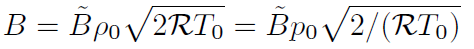
The output values of the simulation saved in the Matlab matrices are a coefficient B_tilde, which has the dimension of a surface (μm^2) and depends only on the problem geometry. The real damping coefficient B can be computed from B_tilde according to:
Pre-computed elemental units
In order to simplify considerably the analysis of the global device, MEMS surfaces can be grouped into typical element units. Here we have considered three elemental blocks: parallel surfaces, comb finger unit and mass with a hole.
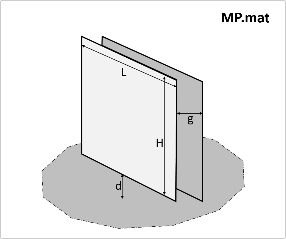
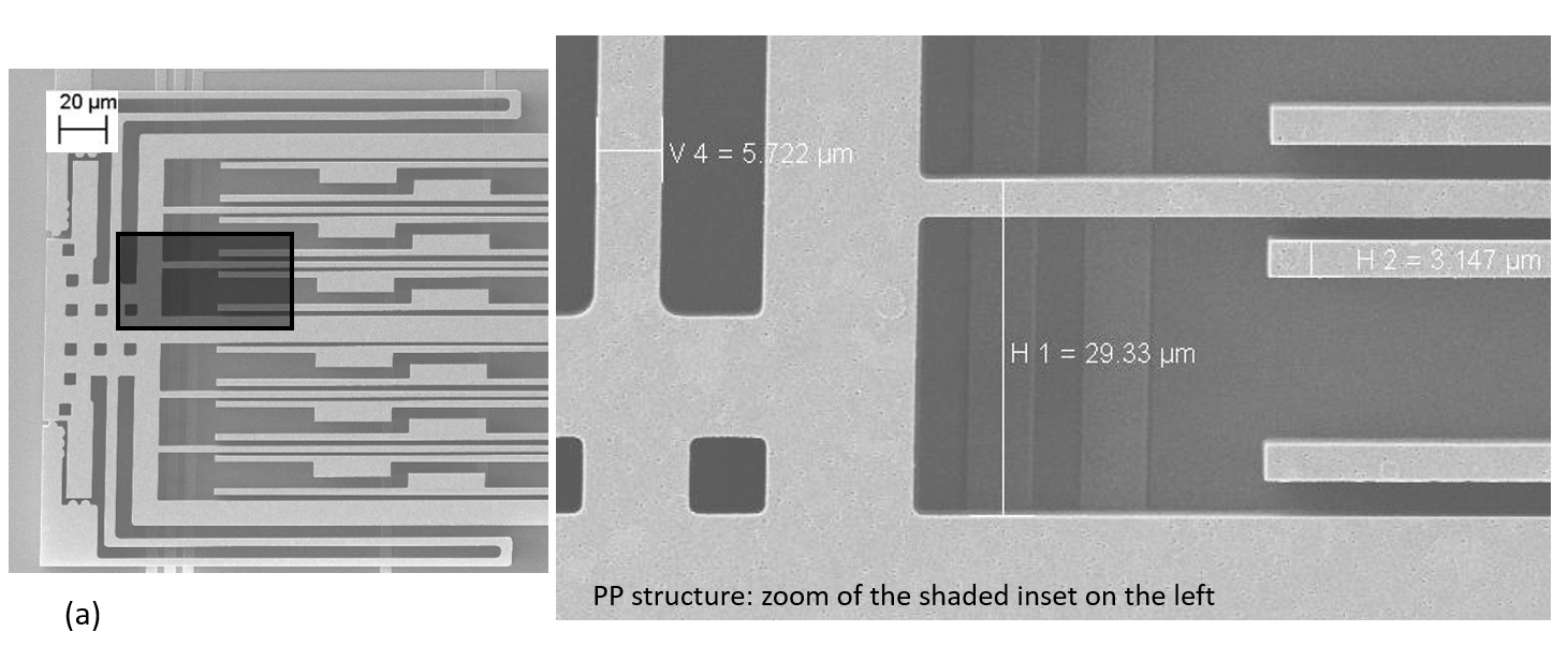
1. Parallel surfaces
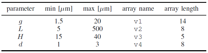
Two rectangular surfaces of dimensions H x L are separated by a gap g and placed over a substrate at distance d. The shuttle surface moves with unit velocity in the direction of the gap towards the fixed surface.
The values of B_tilde are collected in four-dimensional Matlab array MP and saved in a file MP.mat, together with the arrays of parameters.
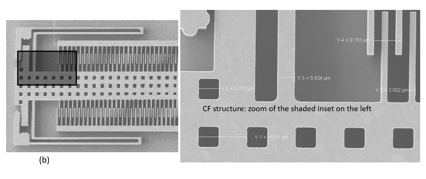
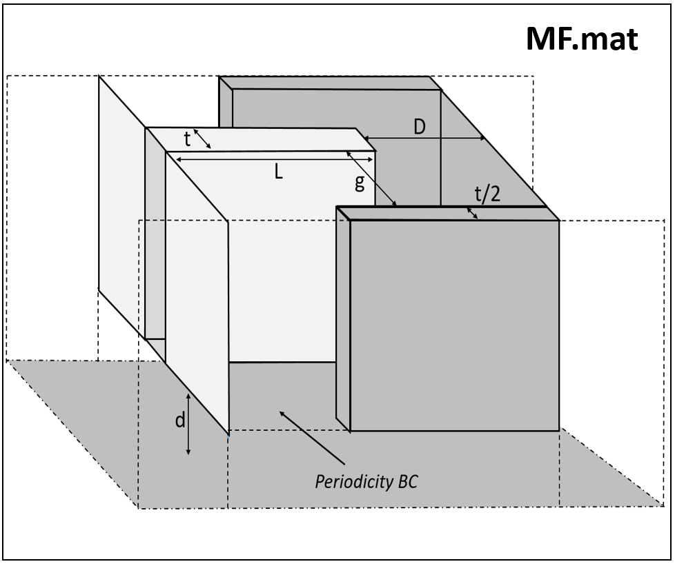
2. Comb finger unit
A shuttle finger of dimensions H x L x t moves with unit velocity in the direction of the finger axis within two identical stator fingers. Shuttle and stator fingers are placed at distance d over a substrate. This unit is conceived as a part of a long set of identical blocks and periodicity boundary conditions are enforced to predict the dissipation of a “regime” unit.
The values of B_tilde are collected in a six-dimensional Matlab array MF and saved in a file MF.mat, together with the arrays of parameters.
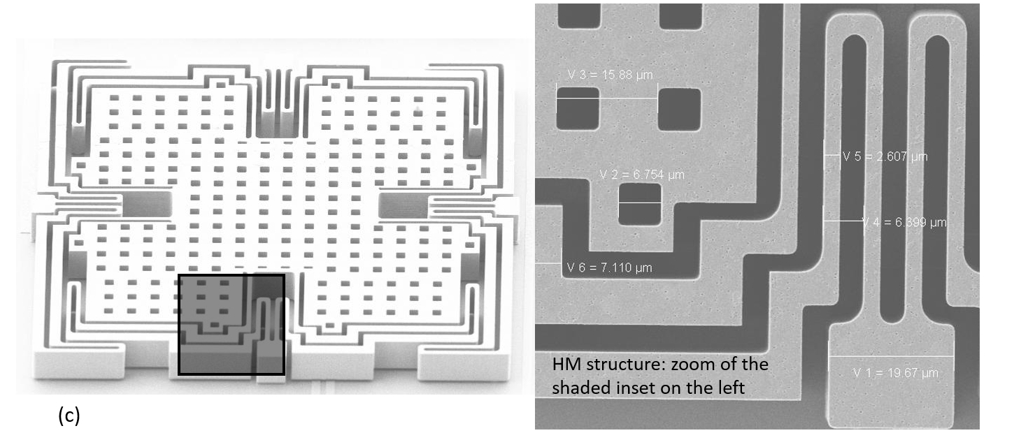
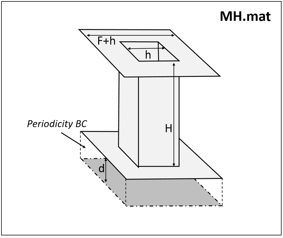
3. Perforated mass (mass with a hole)
A square hole of side h is made in a plate of side h+F and thickness H vibrating with a unit velocity orthogonally to a substrate surface with a gap d. This unit addresses the effects of holes in the out-of-plane vibrations of masses. Periodicity boundary conditions are enforced to predict the dissipation of three levels of holes according to their distance from the border and a “regime” unit.
The values of B_tilde are collected in four four-dimensional Matlab arrays MH1, MH2, MH3, MH and saved in a file MH.mat, together with the arrays of parameters.
Numerical code freemolBIE
A demo serial non-optimized version of the numerical code freemolBIE.zip is distributed in order to estimate the gas dissipation for more general elemental units.
General elemental units
In order to extend the ranges of parameters in elemental units when required, three input files are available.
The files are in the folder input and are saved with a .geo extension. These can be edited with any text editor. They are input files for the Gmsh software which generates the mesh file (it must be downloaded on the local machine).
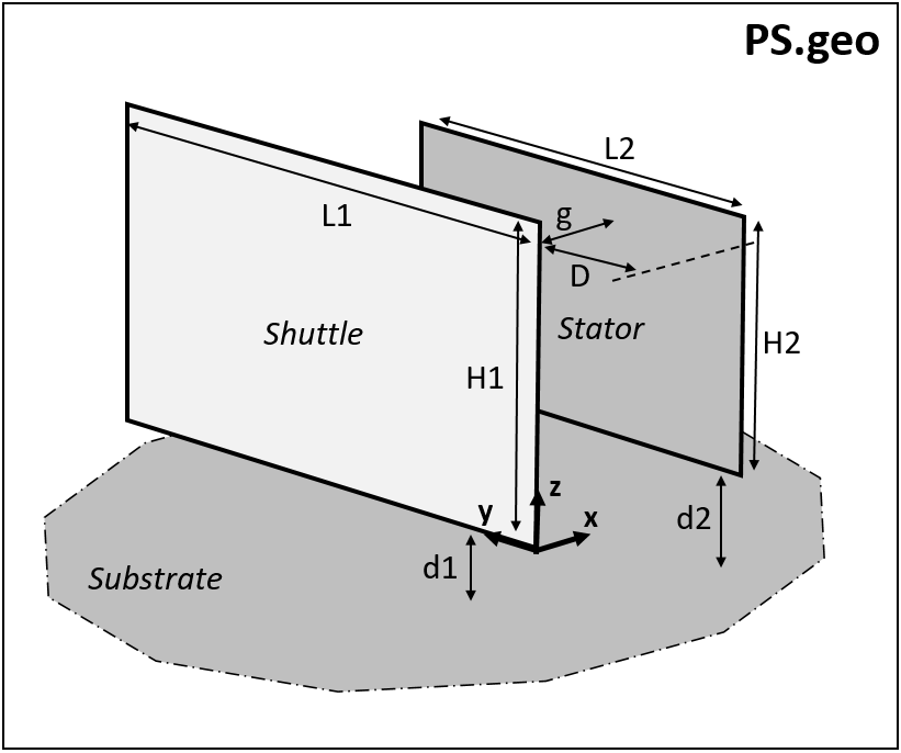
1. Parallel surfaces
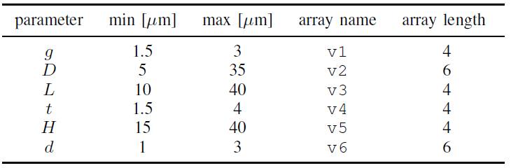
A rectangular surface of dimensions H1 x L1 (shuttle) moves with unit velocity in direction x towards a second fixed parallel rectangular surface (stator) of dimensions H2 x L2 separated by a gap g. The two surfaces are placed over a substrate at distances d1 and d2 respectively.
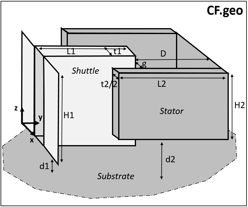
2. Comb finger unit
A shuttle finger of dimensions H1 x L1 x t1 moves with unit velocity in the direction of finger axis y within two stator fingers of dimensions H2 x L2 x t2. Shuttle and stator fingers are placed at distances d1 and d2 respectively over a substrate.
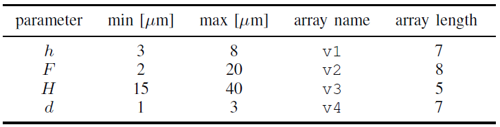
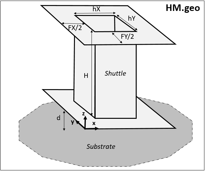
3. Hole
A rectangular hole of dimensions hX x hY is made in a plate of dimensions (hX+FX)x(hY+FY) and thickness of H vibrating in direction z with a unit velocity orthogonally to a substrate surface with a gap d.
Using the code
There are four fundamental steps.
1. Setting the parameters
The first step is to set the parameters in the selected input file. The geo file can be opened with Gmsh to view the layout of the elemental units. Selecting the module Geometry->Edit file a standard text editor opens and the parameters can be modified. After that remember to Reload the file for changes to take effect.
For CF.geo it is possible to choose the number of identical comb finger units, whereas for HM.geo two parameters set the number of identical holes in X and Y directions, respectively.
In all the input files one can fix the extension of the substrate and the level of mesh refinement.
2. Generation of mesh file
Generate with Gmsh the mesh using the module Mesh->2D and then Save it. A .msh file will be generated and represents the real input of freemolBIE.
N.B. Whenever the geo file is modified, the mesh must be regenerated
3. Running of the code
Now the user is ready to launch the code, simply clicking on the executable file freemolBIE.exe.
A DOS-like shell opens and asks for the name of the desired input file.
Finally, the code runs and prints the coefficient B_tilde of the overall shuttle structure.
N.B. The demo serial version made available is not suited for large-scale problems!
4. Output
The code places in the output folder:
1) A txt file with the total structure dissipation and also the contribution of each unit in the case of CF and HM. The output values are the coefficient B_tilde [μm^2]:
2) A geo file with two msh files which plot in Gmsh some geometrical properties, like the normal and velocity vectors, and the results of the simulation: flux j and force vector t.
References
- A. Frangi, Di Gioia A., Multipole BEM for the evaluation of damping forces on MEMS, Computational Mechanics, 37, 24-31, 2005
- A. Frangi, Spinola G., Vigna B., On the evaluation of damping in MEMS in the slip-flow regime, International J. Numerical Methods in Engineering, 68, 1031-1051, 2006
- A. Frangi, A. Frezzotti, S. Lorenzani. On the application of the BGK kinetic model to the analysis of gas-structure interactions in MEMS, Computers & Structures 85, 810-817, 2007.
- A. Frangi, A. Ghisi, L. Coronato. On a deterministic approach for the evaluation of gas damping in inertial MEMS in the free-molecule regime, Sensor & Actuators, A, 149, 21-28, 2009.
- A. Frangi. BEM technique for free-molecule flows in high frequency MEMS resonators, Engineering Analysis with Boundary Elements, 33, 493-498, 2009.
- A. Frangi, G. Laghi, G. Langfelder, P. Minotti, S. Zerbini, Optimization of Sensing Stators in Capacitive MEMS Operating at Resonance, IEEE JMEMS 24 (4), 1077-1084, 2015.
- A. Frangi, P. Fedeli, G. Laghi, G.Langfelder, G.Gattere. Near Vacuum Gas Damping in MEMS: Numerical Modeling and Experimental Validation, IEEE JMEMS, 25 (5), 890-899, 2016.
- P. Fedeli, A. Frangi, G. Laghi, G.Langfelder, G.Gattere. Near Vacuum Gas Damping in MEMS: Simplified Modeling, IEEE JMEMS, 26 (3), pp. 632-642, 2017.